1. Introduction
Traditional databases allows partitioning of large tables where the data in table divided into segments, called partitions, that make it easier to manage and query your data. This is referred to as static partitioning which requires you to include a partitioning clause in the CREATE TABLE statement to create a partitioned table.
The Snowflake Data Platform, as opposed to a traditional data warehouse, uses a unique and distinctive method of partitioning called Micro-partitioning that offers all the benefits of static partitioning without the known drawbacks and offers extra substantial advantages.
2. What are Micro-partitions?
All data in Snowflake is stored in database tables, logically structured as collections of columns and rows. Although this is how the front-end functions, Snowflake does not actually handle and store data in this manner. Instead, Snowflake stores all table data automatically divided into encrypted compressed files which are referred to as Micro-partitions.
Micro-partitions are immutable files i.e. cannot be modified once created and stores data in columnar format. Every new data arrival creates a new micro-partition. Each micro-partition contains between 50 MB and 500 MB of uncompressed data.
Micro-partitioning is automatically performed on all Snowflake tables. The order in which the data is put or loaded is used to transparently partition the tables.
3. Query Pruning
Snowflake also stores metadata about all rows stored in a micro-partition. The metadata information includes
- The range of values for each of the columns in the micro-partition.
- The number of distinct values.
- Additional properties used for both optimization and efficient query processing.
This metadata is an essential component of the Snowflake architecture because it enables queries to decide whether or not to query the data included in a micro-partition. In this manner, only the micro-partitions containing the relevant data are queried when a query is executed, saving time and resources. This process is known as Query Pruning, as the data is pruned before the query itself is executed.
4. How does the organization of data into micro-partitions impact query performance?
The performance of pruning greatly depends on how data is divided into micro-partitions. Let us understand with an example provided by the Snowflake’s own documentation.
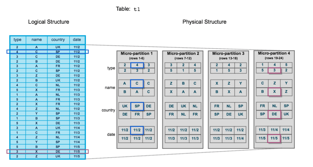
This image may initially be difficult to understand. Let’s analyse it step by step, beginning with the left side. This is the way a table might show up in the Snowflake user interface. This is referred to as the Logical Structure. There are 24 rows of data and 4 columns – type, name, country, and date.
An illustration of how this information would be kept in backend of Snowflake’s architecture can be seen on the right. This is referred to as the Physical Structure. Here, there are four distinct micro-partitions that each hold six rows of data. Data of rows 1 through 6 are contained in the first micro-partition and so on. Since the data is stored in columnar format, Snowflake can retrieve certain columns of data without dissecting individual rows.
Row 2 and row 23 are two particular rows of data that have been highlighted to see how they are stored in logical vs physical structure.
Now consider that you wanted to retrieve records that belong to date ‘11/2’ from the above example.
SELECT type, country FROM MY_TABLE
WHERE Date = '11/2' ;
The data of the records that belong to date ‘11/2’ is present in micro-partitions 1, 2 and 3. Similarly for other dates, the data is spread across micro-partitions is as depicted below.
| Date | Micro-Partitions |
| 11/2 | 1,2,3 |
| 11/3 | 2,3,4 |
| 11/4 | 3,4 |
| 11/5 | 4 |
When you execute this query in Snowflake, only those micro-partitions are scanned which satisfies the filter condition. Once the micro-partitions to be scanned are identified, a portion of the micro-partitions is scanned that contain the data for the columns in the select query so that an entire partition is not scanned
As the query performance is directly linked to the amount of the data that it scans, organizing data in micro-partitions yields better overall performance which could be done using the concept called Data Clustering.
5. What is Data Clustering?
Clustering is a technique used to organize data storage to better accommodate anticipated queries. The key objective is to increase query performance while lowering the amount of system resources needed to run queries.
Snowflake supports explicitly selecting the columns on which a table is clustered, giving you additional control over the clustering process. These columns are known as Clustering keys, and they allow Snowflake to maintain the clustering in accordance with the chosen columns while also allowing you to recluster on demand.
Although clustering can substantially improve the performance and reduce the cost of some queries, the compute resources used to perform clustering consume credits. So, you should cluster only when the table contains multiple terabytes (TB) of data with a large number of micro-partitions and queries will benefit substantially from the clustering.
Let us take the earlier example we discussed and see how clustering the table on date column would have distributed data into micro-partitions using below image.

The below table shows distribution of rows with distinct date values in various micro-partitions. This clearly shows clustering the table on date columns reduced the number of micro-partitions to be scanned than earlier scenario.
| Date | Micro-Partitions |
| 11/2 | 1,2 |
| 11/3 | 3 |
| 11/4 | 4 |
| 11/5 | 4 |
This example is just a simple conceptual representation of the data clustering that Snowflake utilizes in micro-partitions. In real world clustering table with such a small data set would not have any noticeable impact. Extrapolated to a very large table (i.e. consisting of millions of micro-partitions or more), clustering can be very effective.
6. How to create Clustered Tables in Snowflake?
In the above example, we clustered our dataset based on the date field. As we have clustered based on this field, this field is referred to as the clustering key.
A clustering key can be defined when a table is created by appending a CLUSTER BY clause to CREATE TABLE as shown below
CREATE TABLE MY_TABLE (
    type NUMBER
  , name VARCHAR(50)
  , country VARCHAR(50)
  , date DATE
)
CLUSTER BY (date) ;
In the above example we have created a table with clustered key. However you can also cluster a table by specifying a CLUSTER KEY at a later point in time using ALTER TABLE as shown below.
ALTER TABLE MY_TABLE
CLUSTER BY (date) ;
Although we have just used one field as a clustering key in our example, this is not the only choice. A clustering key can be defined using many fields if desired as shown below.
ALTER TABLE MY_TABLE
CLUSTER BY (date, type) ;
Another advantage is that Snowflake also supports expressions on fields in a cluster key. The below example shows the table is clustered using the year of the date field and first two letters of country field.
ALTER TABLE MY_TABLE
CLUSTER BY (YEAR(date), SUBSTRING(country,1,2)) ;
7. Reclustering
A clustered table’s data may become less clustered as DML operations (INSERT, UPDATE, DELETE, MERGE, COPY) are carried out on it. The table must be periodically or regularly reclustered in order to maintain optimal clustering.
Changing the clustering key for a table using ALTER TABLE does not affect existing records in the table until the table has been reclustered by Snowflake.
During reclustering, Snowflake uses the clustering key for a clustered table to reorganize the column data, so that related records are relocated to the same micro-partition. Each time data is reclustered, the rows are physically grouped based on the clustering key for the table, which results in Snowflake generating new micro-partitions for the table.
Reclustering in Snowflake is automatic and no maintenance is needed. However, the rule does not apply to tables created by cloning from a source table that has clustering keys.
This reclustering results in storage costs because the original micro-partitions are marked as deleted, but retained in the system to enable Time Travel and Fail-safe.
The below image shows how reclustering the data on date and type fields creates new micro-partitions based on Clustering key defined.

8. Automatic Clustering
Automatic Clustering is the Snowflake service that seamlessly and continually manages all reclustering, as needed, of clustered tables. Note that Automatic Clustering consumes Snowflake credits, but does not require you to provide a virtual warehouse. Instead, Snowflake internally manages and achieves efficient resource utilization for reclustering the tables.
To suspend Automatic Clustering for a table, use the ALTER TABLE command with a SUSPEND RECLUSTER clause. For example:
ALTER TABLE my_table
SUSPEND RECLUSTER ;
To resume Automatic Clustering for a clustered table, use the ALTER TABLE command with a RESUME RECLUSTER clause. For example:
ALTER TABLE my_table
RESUME RECLUSTER ;
Verify if Automatic Clustering is enable for a table using SHOW TABLES command.
SHOW TABLES LIKE 'my_table';9. Clustering Information
Snowflake has provided a system function named SYSTEM$CLUSTERING INFORMATION to help in determining how well-clustered a table is. This function accepts a table name and a list of columns as inputs and returns a summary of how well the table is clustered based on the list of columns.
If no list of columns is provided, the function will instead return the clustering information for the table based on its current clustering key. If no current clustering key is defined on the table, the function will error.
The syntax to execute the function is as shown below
SELECT SYSTEM$CLUSTERING_INFORMATION('my_table', '(date, type)');The function returns a JSON object containing the following name/value pairs:
9.1. cluster_by_keys
- Columns in table used to return clustering information. The columns which you pass as arguments to the function.
9.2. total_partition_count
- Total number of micro-partitions that comprise the table.
9.3. total_constant_partition_count
- Total number of micro-partitions for which the value of the specified columns have reached a constant state i.e. the micro-partitions will not benefit significantly from reclustering. As this number increases, we can expect query pruning to improve and queries to execute more efficiently.
9.4. average_overlaps
- The term “Overlap” indicates the number of partitions which share the same specified column value.
- For each micro-partition in the table, this gives the average number of overlapping micro-partitions. A high number indicates the table is not well-clustered.
9.5. average_depth
- The term “Depth” indicates the number of partitions in which same column value exists when an overlap occurs.
- For each micro-partition in the table, this gives the average overlap depth. A high number indicates the table is not well-clustered.
- This value is also returned by SYSTEM$CLUSTERING_DEPTH.
9.6. partition_depth_histogram
- A histogram depicting the distribution of overlap depth for each micro-partition in the table. The histogram contains buckets with widths:
- 0 to 16 with increments of 1.
- For buckets larger than 16, increments of twice the width of the previous bucket (e.g. 32, 64, 128, …).
I have included below an example provided by snowflake showing output of system$clustering_information
{
    "cluster_by_keys" : "(COL1, COL3)",
    "total_partition_count" : 1156,
    "total_constant_partition_count" : 0,
    "average_overlaps" : 117.5484,
    "average_depth" : 64.0701,
    "partition_depth_histogram" : {
                  "00000" : 0,
                 "00001" : 0,
                 "00002" : 3,
                 "00003" : 3,
                 "00004" : 4,
                 "00005" : 6,
                 "00006" : 3,
                 "00007" : 5,
                 "00008" : 10,
                 "00009" : 5,
                 "00010" : 7,
                 "00011" : 6,
                 "00012" : 8,
                 "00013" : 8,
                 "00014" : 9,
                 "00015" : 8,
                 "00016" : 6,
                 "00032" : 98,
                 "00064" : 269,
                 "00128" : 698
    }
}
This might be a lot of information to take in at the moment. But based on data do you think the table is well clustered?
To answer the question, every metric indicates that the table is not well clustered. The metric values which are expected to be high are low and vice versa.
For more information refer this Snowflake Documentation.
10. Conclusion
This article is extensive and covers a wide range of topics related to micro-partitions and clustering. However, in order to have a thorough understanding, I felt it was necessary to discuss all of these topics in one article. I would recommend playing around with the functionality to better understand the concepts. Make use of Snowflake sample database and cloning functionalities to create tables with larger data and see how query performance varies using various clustering keys.
Subscribe to our Newsletter !!
Related Articles:

There are three different types of views in Snowflake – Non-Materialized, Materialized and Secure Views.
Secure Data Sharing in Snowflake enables account-to-account sharing of selected database objects in your account with other.
A Stream is a Snowflake object that provides change data capture (CDC) capabilities to track the changes in a table.